Most of our statistical evaluations rely on the Cumulative Distribution Function (CDF). Even though a histogram seems to be more intuitive at the first look and needs less explanation, in practice the CDF offers a couple of advantages, which make it worth getting acquainted with it. The main advantages of the CDF and the reasons why we primarily use it instead of the histogram are listed in the following after a principal explanation of both plots.

Basic Description

Before exploring the advantages of the different plots, they are first described here.

A set of numbers should be given. These can come from any type of measurements, simulations, or arbitrary other data sources. Simply for illustration we just produced some normally distributed numbers with the MATLAB random number generator:

x=randn(100,1)*10+50

Showing these numbers with the help of a histogram, the resulting range of the numbers is split into a certain amount of uniform intervals – so-called bins. Then the absolute or relative count of numbers within each bin is plotted as a bar at the according intervals. The result for the previous example may look like the following plot:

On the other side, in the Cumulative Distribution Function (CDF) the percentage or relative count of the sorted numbers is plotted over the numbers themselves. This is more or less the integral of the histogram.

The previous exemplary numbers result in the following diagram:

This plot means that a relative amount of F(x) values from the given set of numbers are less or equal than the value x.

In our opinion this diagram has a lot of essential advantages.

Direct Quantitative Reading of Essential Key Values

One of the main advantages of the CDF with respect to the histogram is the fact that main and important key values and features like minimum, maximum, median, quantiles, percentiles, etc. can be directly read from the diagram.

The minimum can be seen right at the point where the CDF begins and hits the x-axis. The maximum can be seen where the CDF reaches the line y=1 and ends. Percentile and quantiles can also be read directly from the x-axis.

Each value from the given set of numbers is a certain point in the CDF. In some of our CDF evaluation we have implemented that the point is named or its values are shown directly, when clicking on that point in the CDF. In the histogram the number samples cannot be addressed individually.

Detection of Outliers

In some cases the detection of outliers may become problematic with the histogram. As an example we have added the value 400 to the given exemplary numbers from above. The corresponding histogram looks like this:

In case the data set is quite big the outlier may not be seen well due to the relative small relation to the total number of values. On the other side the outlier stretches the size of the bins in a way that the original distribution may become hard to recognize. Therefore the number of bins would have to be extended according the distance of the outlier to the main values. But this can normally only be done well afterwards and not a priori or would require some sophisticated algorithms for the selection of the bin size. If the limits of the x-axis is not changed according the outlier, the outlier may also be overseen at all. The histogram gives no indication that there is still data existing outside the displayed axis limits.

Within the cumulative distribution function outliers can be seen through the tails of the CDF curve. Their value is directly visible at the end of the tail. Also the type of the distribution stays visible even with the rescaling of the x-axis as caused by the outlier.

If the limits of the x-axis are not changed to accomodate all data, the existence of an outlier would still stay evident, due to the fact that the distribution function does not end before the axis limit and does not reach the line y=1.

Display of Infinity Values

If some infinity values are part of the data set, their existence cannot be seen in the histogram at all. In the CDF the existence of infinity values can be seen because the plot does not reach the lower line y=0 (for -Inf)or the upper line y=1 (for +Inf). The distance from the end of the CDF to the upper and lower lines also indicates the relative number of infinity values. This is true for negative infinities as well as for positive ones. Sometimes we mark these with circles for highlighting and easying the recognition of such values.

Identification of the Distribution Type

We agree that the identification of the type of a distribution may be simpler by the use of a histogram. Within the histogram one can easily recognize if the data is normally distributed or follows any different distribution type. On the other side one can directly apply the Kolmogorov Smirnov test if not only the empirical distribution function itself but also the CDF of the expected distribution type is plotted (compare the red line for a normal distribution in the following diagram). The maximum distance of these two curves in the y-direction verifies the type of the distribution. The smaller this difference is, the more evidence about the distribution type is given.

Identification of Clusters

Like for distribution types, the existence of clusters can be seen easily within the histogram.

But clusters can also be seen in the CDF clearly with only little practice. One only has to look for decreasing slope, where the gradient increases again later. An example can be seen in the next diagram, which relies on the same numbers than the histogram above.

Comparison of Several Data Sets

The CDF is much more suitable for comparisons of several data sets than a histogram. An arbitrary number of CDFs can be plotted into the same axes without any problems for comparisons. Hereby it is irrelevant how much data each set actually contains.

Histograms quickly become confusing and the different data sets can hardly be distinguished visually. Beside all the other disadvantages of the histogram, these are also much more complicated to produce here. For example all the bins have to be synchronized for all the data sets. This may even worsen the existing disadvantages of the histograms.

Safety Against Misinterpretation and Manipulation

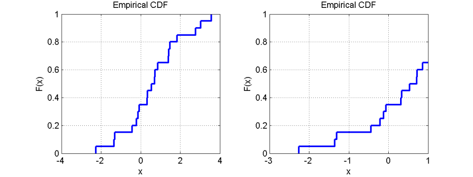
A further disadvantage of the histogram is its sensitivity with respect to some display parameters, like the bin size. Take the example of the following normally distributed data set, which has been generated again by the MATLAB random number generator (randn(20,1)):

[0.5377, 0.5377, 1.8339, -2.2588, 0.8622, 0.3188, -1.3077, -0.4336, 0.3426, 3.5784, 2.7694, -1.3499, 3.0349, 0.7254, -0.063, 0.7147, -0.2050, -0.1241, 1.4897, 1.4090, 1.4172]

Depending on the chosen number of bins the resulting diagrams may differ significantly:

The histogram with 5 bins correlates largely with the expected normal distribution. The same numbers look completely different, when 6 bins are selected for illustration. In that case the histogram looks like a multimodal distribution with 3 clusters instead of a normal distribution.

In the case that axis limits are selected unluckily, the picture becomes even worse:

Contrary to that the display of the CDF is always clear and unique. If the axis limits are defined within the range of the data set, the CDF does not reach the lines y=0 or y=1. This clearly indicates that there is some more data available that cannot be seen in the current view. That way the CDF is much more robust against “manipulation” and misinterpretation due to unlucky display parameters.